
Excel library
How to Sum a Column Based on Another Column Value in Excel?
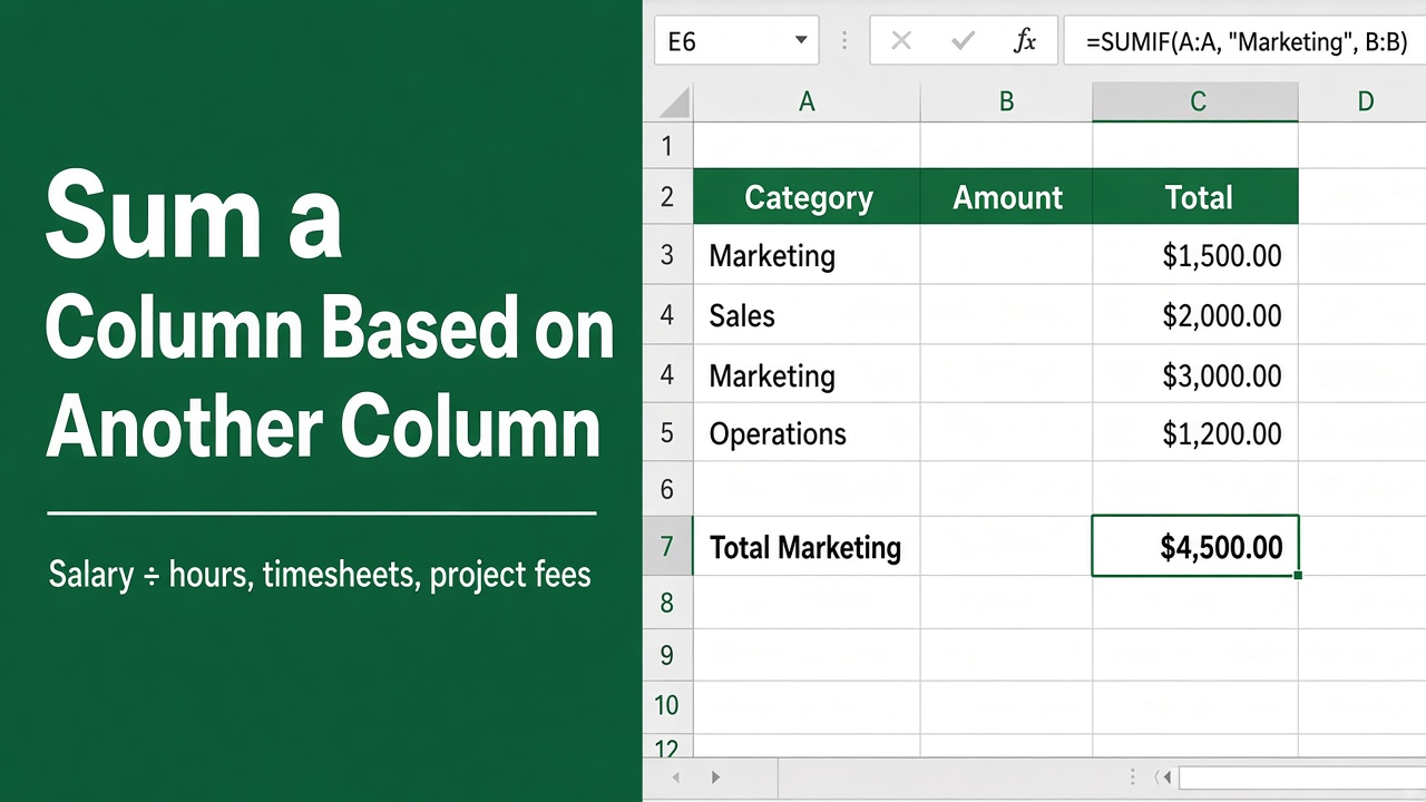
When working with data in Microsoft Excel, you may need to add numbers only when another column contains a specific value. For example, you might want to calculate total sales for a particular product, add expenses from one category, or sum orders handled by a specific employee.
The easiest way to sum a column based on another column value in Excel is to use the SUMIF function. For more complex conditions, you can use SUMIFS, SUMPRODUCT, or other Excel formulas.
How to Sum a Column Based on Another Column Value in Excel Using SUMIF
The SUMIF function is usually the best option when you have one condition. It checks one range for a specific criterion and then adds the corresponding values from another range.
The SUMIF syntax is:
=SUMIF(range, criteria, sum_range)Here is what each argument means:
| Argument | Purpose |
|---|---|
| range | Cells Excel checks against your condition |
| criteria | The value or condition you want to match |
| sum_range | Cells containing the numbers to add |
SUMIF Example
Suppose you have this sales data:
| Product | Sales |
|---|---|
| Laptop | 800 |
| Mouse | 100 |
| Laptop | 650 |
| Keyboard | 150 |
| Laptop | 900 |
To calculate the total sales for Laptop, enter:
=SUMIF(A2:A6,"Laptop",B2:B6)Excel checks cells A2:A6 for the word “Laptop.” Whenever it finds a match, it adds the corresponding value from column B.
The result is:
2,350
This is one of the simplest ways to sum values based on criteria in Excel.
Sum Based on a Value Stored in Another Cell
You do not have to type the criterion directly into your formula. Instead, you can reference another cell.
For example, suppose D2 contains:
LaptopYou can use:
=SUMIF(A2:A6,D2,B2:B6)Now the formula uses the value in cell D2 as the criteria.
This method is useful when creating reports, dashboards, and reusable worksheets because you can change D2 without editing the formula.
Sum a Column Based on Multiple Conditions With SUMIFS
The SUMIFS function is useful when your calculation depends on two or more conditions.
Its basic syntax is:
=SUMIFS(sum_range, criteria_range1, criteria1, criteria_range2, criteria2)Imagine your worksheet contains:
| Product | Region | Sales |
|---|---|---|
| Laptop | East | 800 |
| Laptop | West | 650 |
| Mouse | East | 100 |
| Laptop | East | 900 |
| Keyboard | West | 150 |
If you want to sum Laptop sales in the East region, use:
=SUMIFS(C2:C6,A2:A6,"Laptop",B2:B6,"East")The result is:
1,700
Unlike SUMIF, SUMIFS supports multiple criteria, making it useful for analyzing larger datasets.
Sum a Column Based on Numeric Criteria
Excel can also sum values when another column meets a mathematical condition.
Suppose column A contains quantities and column B contains sales. To add sales where the quantity is greater than 10, you can use:
=SUMIF(A2:A20,">10",B2:B20)Common Excel criteria operators include:
| Criteria | Meaning |
|---|---|
">10" | Greater than 10 |
"<10" | Less than 10 |
">=10" | Greater than or equal to 10 |
"<=10" | Less than or equal to 10 |
"<>10" | Not equal to 10 |
"=10" | Equal to 10 |
When using comparison operators inside SUMIF, place the condition inside quotation marks.
Combine an Operator With a Cell Reference
If your comparison value is stored in D2, use:
You can also check if one value exists in another column.
=SUMIF(A2:A20,">"&D2,B2:B20)The ampersand (&) joins the greater-than operator with the value stored in D2.
Sum Based on Partial Text
SUMIF also supports wildcards, which are useful when cells contain longer text strings.
The asterisk (*) represents any number of characters.
For example:
=SUMIF(A2:A20,"*Laptop*",B2:B20)This formula sums values from column B when cells in column A contain “Laptop” anywhere in the text.
It could match values such as:
- Gaming Laptop
- Laptop Accessories
- Dell Laptop
- Laptop Stand
You can also use the question mark (?) wildcard to represent a single character.
Sum Values That Do Not Match a Specific Value
Sometimes you need the opposite calculation.
For example, to add all sales except those associated with Laptop, use:
=SUMIF(A2:A20,"<>Laptop",B2:B20)The <> operator means not equal to.
You can also reference a cell:
=SUMIF(A2:A20,"<>"&D2,B2:B20)This makes the formula more flexible when your exclusion criteria may change.
Use SUMPRODUCT for More Flexible Conditional Sums
The SUMPRODUCT function provides another way to perform conditional calculations.
For example:
=SUMPRODUCT((A2:A20="Laptop")*B2:B20)The expression:
A2:A20="Laptop"creates a set of TRUE and FALSE results. Excel effectively converts matching entries into 1 and non-matching entries into 0. SUMPRODUCT then multiplies these values by the corresponding numbers in column B and calculates the total.
SUMPRODUCT can be useful when you need advanced conditional calculations that are difficult to handle with a standard SUMIF formula.
SUMIF vs SUMIFS vs SUMPRODUCT
Choosing the right Excel function depends on the type of calculation you need.
| Function | Best Use |
|---|---|
| SUMIF | Sum based on one condition |
| SUMIFS | Sum based on multiple conditions |
| SUMPRODUCT | More complex conditional calculations |
| SUM | Add values without conditions |
For most worksheets, start with SUMIF for a single criterion and SUMIFS when multiple criteria are required.
Common SUMIF Problems and How to Fix Them
If your SUMIF formula returns an incorrect result, first check that the criteria range and sum range cover the correct rows.
For example:
=SUMIF(A2:A100,"Laptop",B2:B50)uses ranges of different sizes and can produce unexpected results. A better formula is:
=SUMIF(A2:A100,"Laptop",B2:B100)You should also check for extra spaces, numbers stored as text, incorrect comparison operators, and inconsistent data.
For text criteria, make sure the spelling matches your source data. Wildcards can help when you need to match only part of a text string.
Using Excel Tables for Conditional Sums
If your data changes regularly, consider converting the range into an Excel Table using Ctrl + T.
Suppose your table is named SalesData and contains columns called Product and Sales. You could write:
=SUMIF(SalesData[Product],"Laptop",SalesData[Sales])Structured references make formulas easier to understand and automatically adjust when new rows are added to the table.