
Excel library
How to Find the Range in Excel (3 Easy Formulas)
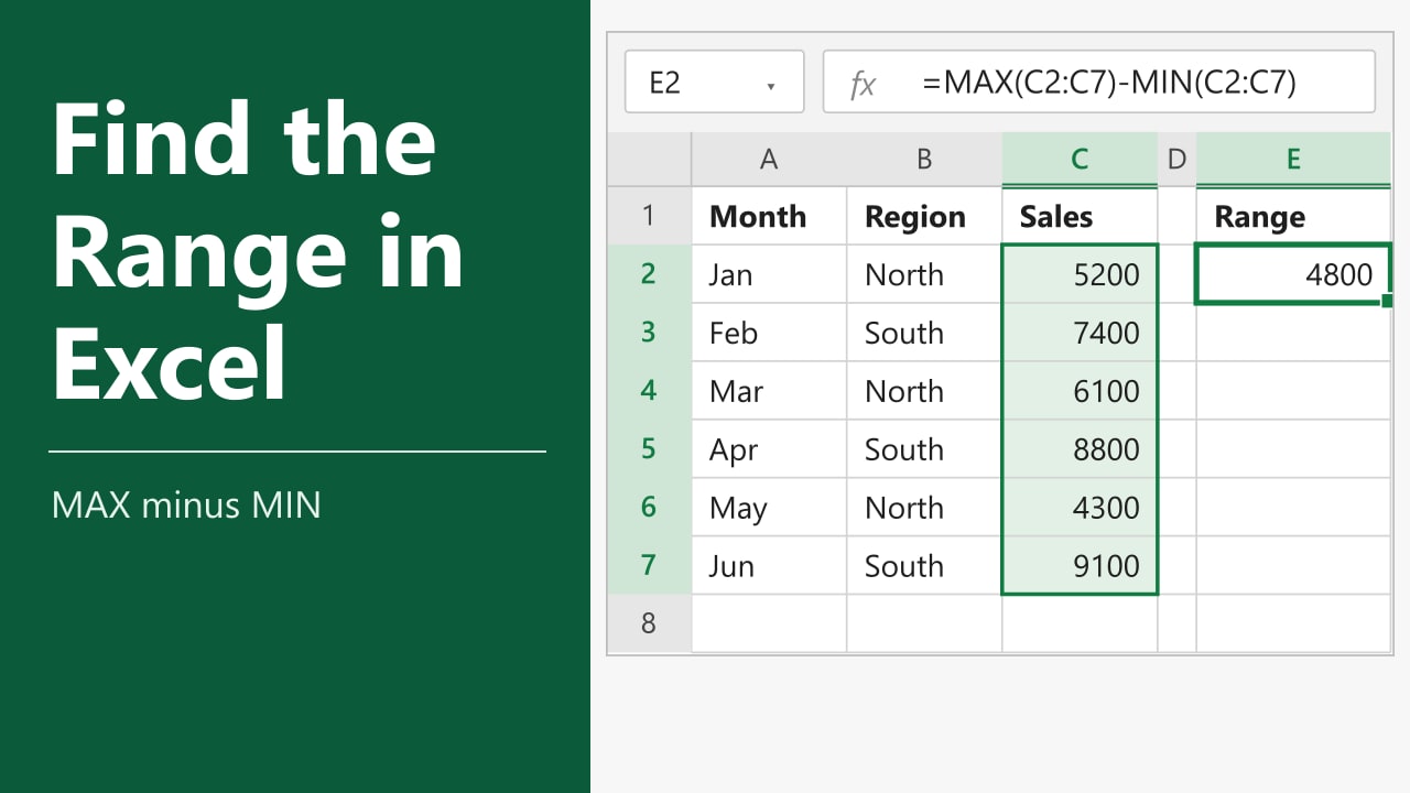
You have a column of sales figures and you want to know how far apart your best and worst results are. That gap is the range: the highest value minus the lowest value. In this tutorial, I'll show you how to find the range in Excel with three formulas: one for a plain list, one for filtered rows and one for each group in your data.
- Click an empty cell, such as E2.
- Type
=MAX(C2:C7)-MIN(C2:C7), using your own cell range. - Press Enter. The cell shows the range.
For filtered rows use Method 2, and for a separate range per group use Method 3.
What Is Range in Excel?
In statistics, the range tells you how spread out your numbers are. You calculate it as highest value - lowest value. Excel does not have a built-in RANGE function for this, so you build it from two functions you probably already know.
This article is about the statistical range. If you meant a cell range such as A1:C7, see how to create a dynamic named range in Excel instead.
All three methods use the same table of monthly sales. Month is in column A, Region in column B and Sales in column C, with the data in A1:C7.
Method 1: Using the MAX and MIN Functions
Use this method when you want the range of every number in a list. It works in every version of Excel.
- Select cell E2, where you want the range to appear.
- Type the formula below.
- Press Enter.
=MAX(C2:C7)-MIN(C2:C7)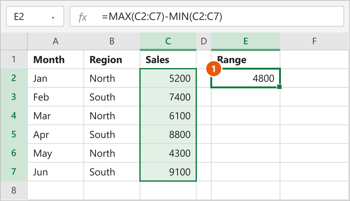
How This Formula Works
MAX(C2:C7) returns the largest sales figure, which is 9100. MIN(C2:C7) returns the smallest, which is 4300. Excel subtracts the second from the first: 9100 - 4300 = 4800.
Note: MAX and MIN ignore empty cells, text and TRUE or FALSE values in the range. If any cell in the range holds an error such as #N/A, the formula returns that error too.
Show the Highest, Lowest and Range Separately
If you want to see the two values behind the range, put each in its own cell. Enter =MAX(C2:C7) in F1 and =MIN(C2:C7) in F2. Then enter the formula below in F3.
=F1-F2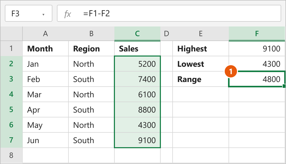
This takes more cells, but readers can check each number at a glance. It is a good layout for a report.
Method 2: Using SUBTOTAL to Find the Range of Filtered Rows
MAX and MIN include rows you have hidden with a filter. Use SUBTOTAL when you want the range of only the rows you can see.
- Select any cell in your table, then press Ctrl + Shift + L on Windows, or go to Data > Filter.
- Click the drop-down arrow in the Region header.
- Clear the South box so only North stays ticked, then click OK.
- Select cell E2 and type the formula below.
- Press Enter.
=SUBTOTAL(104,C2:C7)-SUBTOTAL(105,C2:C7)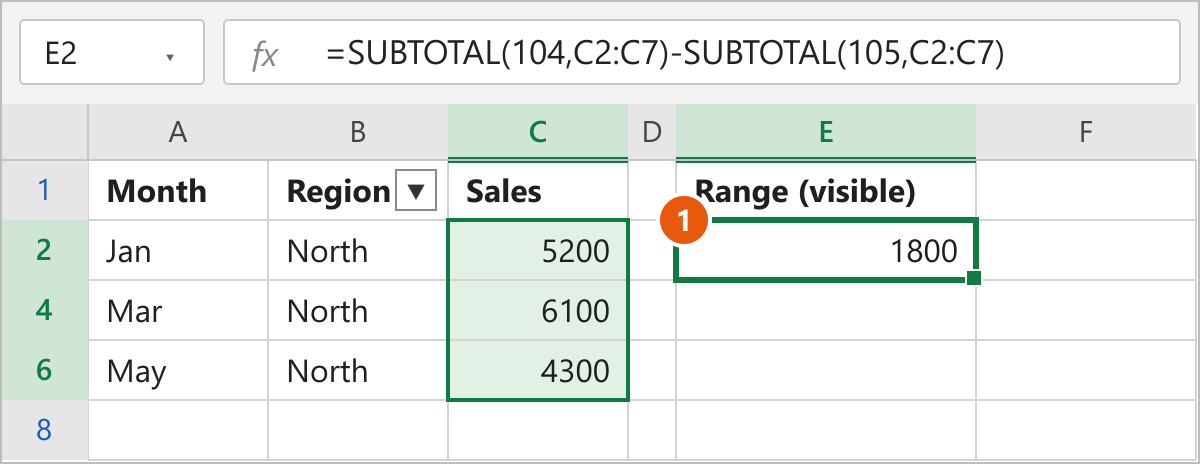
How This Formula Works
The number 104 tells SUBTOTAL to find the maximum, and 105 tells it to find the minimum. Both ignore rows hidden by a filter. The visible North sales are 5200, 6100 and 4300, so the range is 6100 - 4300 = 1800. Change the filter and the result updates on its own.
Note: Put the formula in a row the filter cannot hide, such as above the table. A filter hides entire rows, so if the formula sits in a row that gets filtered out, you will not see the result.
Method 3: Using MAXIFS and MINIFS to Find the Range by Group
Use this method when you want a separate range for each category, such as each region. MAXIFS and MINIFS are available in Excel 2019, Excel 2021 and Microsoft 365, but not in Excel 2016 or earlier.
- In E2 and E3, type the region names North and South.
- Select cell F2.
- Type the formula below.
- Press Enter, then drag the fill handle down to F3.
=MAXIFS($C$2:$C$7,$B$2:$B$7,E2)-MINIFS($C$2:$C$7,$B$2:$B$7,E2)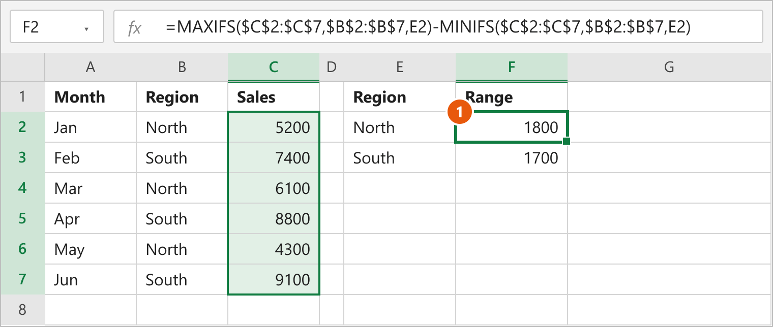
How This Formula Works
MAXIFS returns the largest value in C2:C7 where the region in B2:B7 matches the name in E2. MINIFS does the same for the smallest value. For North, the highest is 6100 and the lowest is 4300, so the range is 1800. For South, it is 9100 - 7400 = 1700.
The dollar signs lock the ranges so they stay in place when you fill the formula down. The E2 reference changes to E3 for the South row.
Note: If no row matches the region name, MAXIFS and MINIFS return 0, so the range shows 0. Check the spelling of the name if you see that.
FAQs
Is there a RANGE function in Excel?
How do I find the range of several columns?
How do I find the range without the highest and lowest values?
Why does my range formula return 0?
Can the range be negative?
Conclusion
For most lists, =MAX()-MIN() is all you need. I'd use it first, and switch to SUBTOTAL when you filter your data often, or to MAXIFS and MINIFS when you want one range per category. Once you have the range, you can look at how values are spread with the standard deviation formula or the median formula.