
Excel library
How to Split Text into Multiple Rows in Excel (3 Easy Ways)
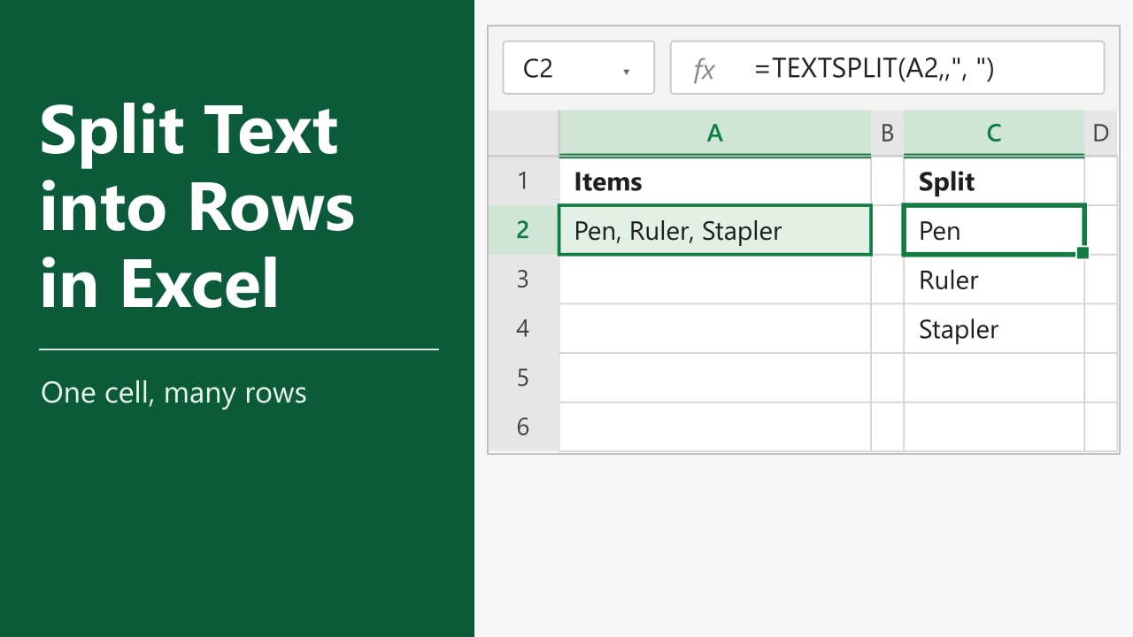
You have a cell with several items packed inside it, such as Pen, Ruler, Stapler, and you need each item on its own row. Doing that by retyping is slow and easy to get wrong. In this tutorial, I'll show you how to split text into multiple rows in Excel with a formula, with Power Query and with Text to Columns plus Transpose.
- Select an empty cell, such as D2.
- Type
=TEXTSPLIT(B2,,", "), replacing B2 with the cell you want to split. - Press Enter. Each item spills into its own row below.
TEXTSPLIT needs Microsoft 365 or Excel 2024. For older versions, use Method 3.
Our Example Data
All three methods use the same small order list. The order numbers are in A2:A4 and the items for each order are in B2:B4, separated by a comma and a space. For example, B2 holds Pen, Ruler, Stapler.
The comma and space is the delimiter, the character that marks where one item ends and the next begins. Your own data might use a semicolon, a dash or a line break instead, and every method below can handle that.
Method 1: Using the TEXTSPLIT Function
Use this method when you have Microsoft 365 or Excel 2024. It is the shortest option, and the result updates when the source text changes.
- Select cell D2, where you want the first item to appear.
- Type the formula below.
- Press Enter.
=TEXTSPLIT(B2,,", ")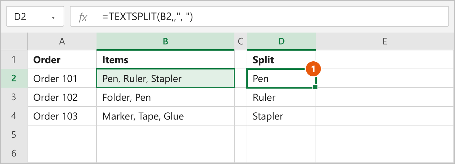
How This Formula Works
TEXTSPLIT takes the text and splits it wherever it finds a delimiter. Its syntax is TEXTSPLIT(text, col_delimiter, [row_delimiter]). The second argument splits text across columns, and the third splits it down rows.
Here, the second argument is left empty and the delimiter ", " goes in the third. That tells Excel to put each piece on a new row. The result is a spill range: you type the formula once in D2 and Excel fills D3 and D4 by itself.
Note: Keep the cells below the formula empty. If something blocks the spill range, Excel returns a #SPILL! error.
Split All the Cells into One Column
The formula above handles one cell. To split every cell in B2:B4 into a single list, first join the cells into one string with TEXTJOIN, then split it.
=TEXTSPLIT(TEXTJOIN(", ",TRUE,B2:B4),,", ")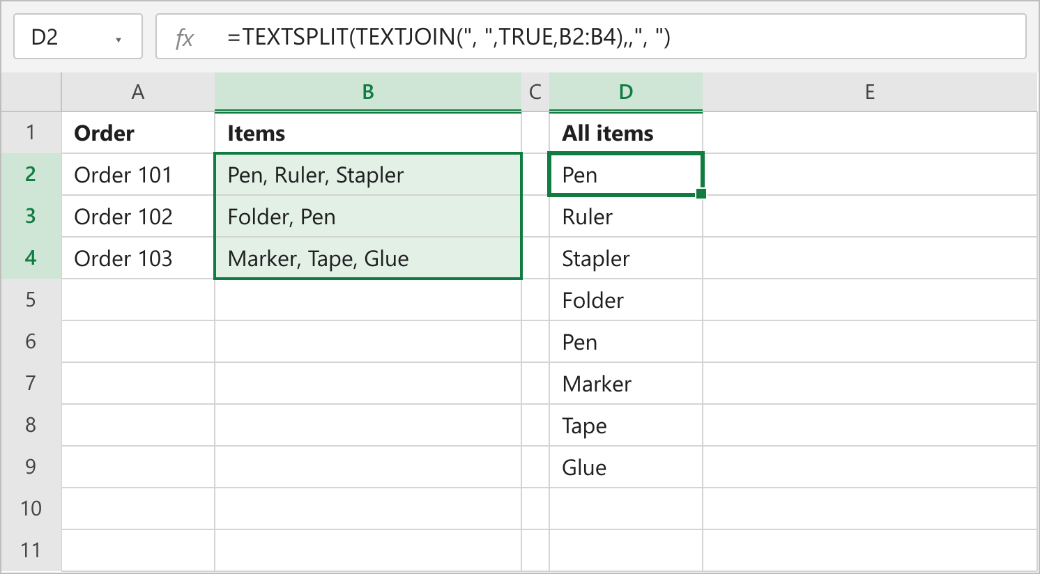
TEXTJOIN glues the three cells into Pen, Ruler, Stapler, Folder, Pen, Marker, Tape, Glue, and TEXTSPLIT then breaks that string into eight rows. This version does not carry the order numbers along. If you need them, use Method 2.
Other Delimiters
Change the third argument to match your data. A few examples:
- For a comma with no space, use
=TEXTSPLIT(B2,,","). - For a line break inside the cell, use
=TEXTSPLIT(B2,,CHAR(10)). - For two different delimiters, use an array:
=TEXTSPLIT(B2,,{",",";"}).
If you are not sure how a line break gets into a cell, see how to insert a carriage return in an Excel cell.
Method 2: Using Power Query
Use this method when you have many rows and want to keep the order number next to each item. Power Query repeats the other columns for every new row it creates. It is built into Excel 2016 and later.
- Select any cell in your data, such as A1.
- Go to the Data tab and click From Table/Range.
- If Excel asks to create a table, check My table has headers and click OK. The Power Query Editor opens.
- Click the Items column header to select it.
- On the Home tab, click Split Column and choose By Delimiter.
- In the Select or enter delimiter list, choose Custom and type a comma followed by a space.
- Expand Advanced options, select Rows under Split into, and click OK.
- On the Home tab, click Close & Load.
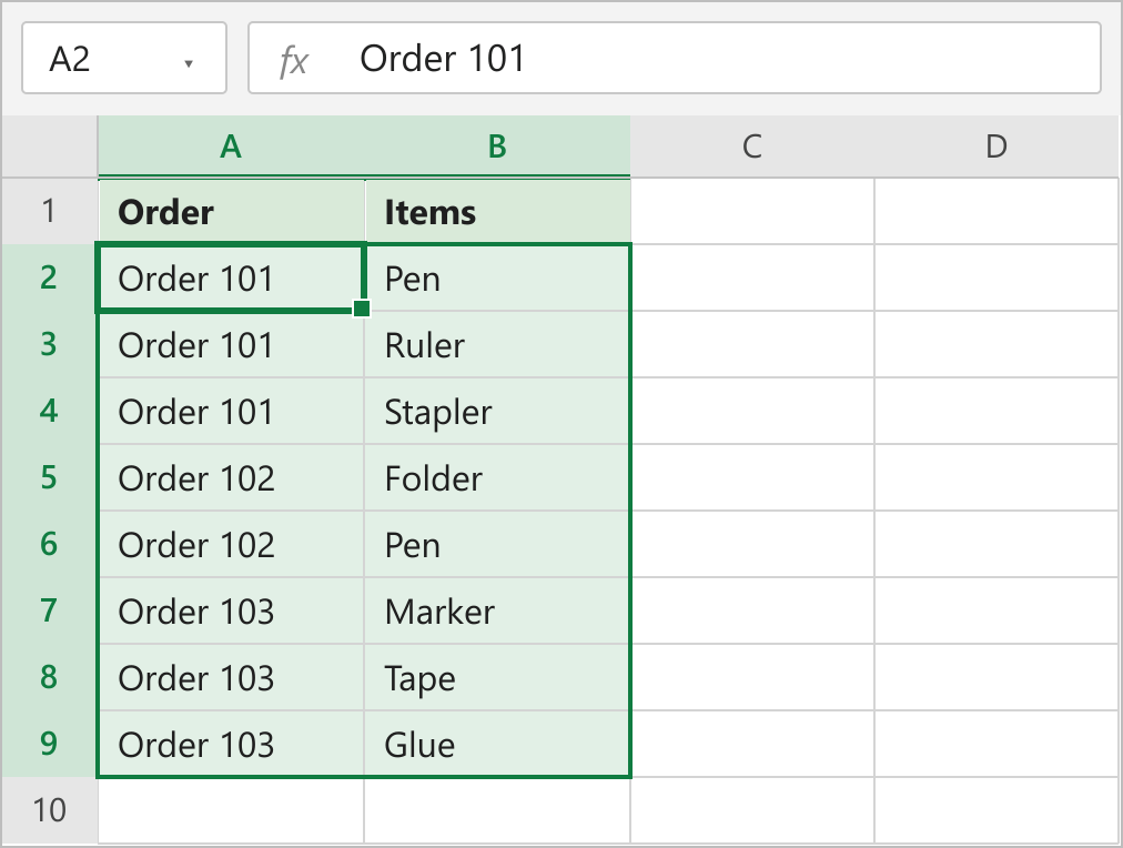
How This Works
The Rows option makes Power Query create a new row for every piece of text it finds, instead of a new column. The Order value is copied onto each new row, so you can still tell which order every item came from. Excel loads the result into a new worksheet as a table.
Note: The output does not update on its own. After you change the source data, right-click the result table and choose Refresh, or go to Data and click Refresh All. If some cells use a comma without a space, the items can carry a leading space. Select the column in the editor and use Transform > Format > Trim to remove it.
Method 3: Using Text to Columns and Transpose
Use this method in older versions of Excel, or when you only need to split one cell. Text to Columns splits the text across a row, and Transpose turns that row into a column.
- Select cell B2.
- Go to the Data tab and click Text to Columns.
- Choose Delimited and click Next.
- Check Comma and Space, check Treat consecutive delimiters as one, and click Next.
- In the Destination box, type
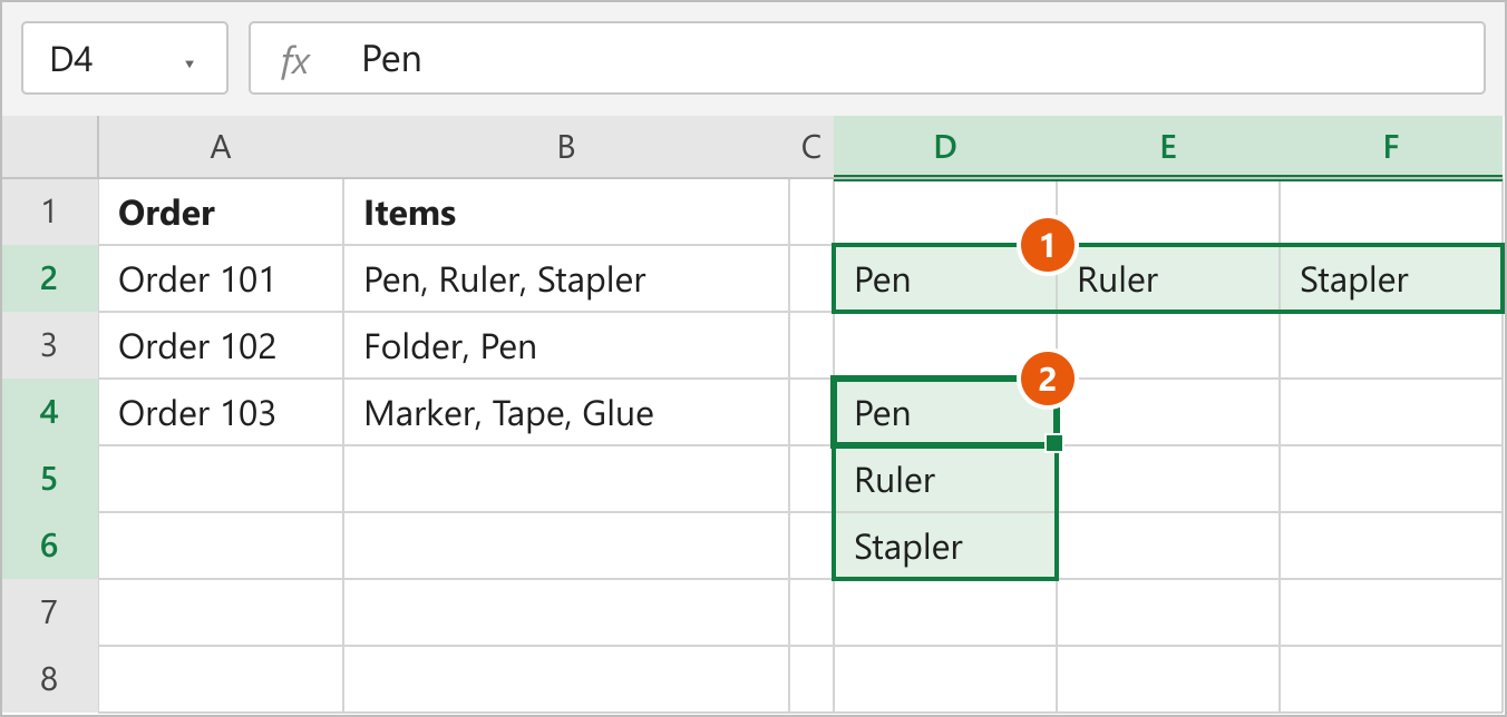
$D$2and click Finish. The items appear across D2:F2. - Select D2:F2 and press Ctrl+C.
- Right-click cell D4 and, under Paste Options, choose Transpose.
How This Works
Typing a destination in step 5 keeps your original text in B2 intact. Without it, Text to Columns overwrites the original cell. The Transpose paste option then flips the three cells in D2:F2 into D4:D6. Once you have the column, you can delete D2:F2. For more on flipping data, see the shortcut for transpose in Excel.
Note: Checking Space also splits items that contain spaces, such as Paper Clip. If your items have spaces, check only Comma and clean up the leading spaces afterward with the TRIM function. Also, the result is static text, so it will not change if you edit the original cell.
Which Method Should You Use?
| Method | Best for | Updates automatically |
|---|---|---|
| TEXTSPLIT | Quick splits in Microsoft 365 or Excel 2024 | Yes |
| Power Query | Many rows, keeping other columns | After a refresh |
| Text to Columns and Transpose | One cell, any Excel version | No |
FAQs
Why does TEXTSPLIT show a #NAME? error?
How do I split text into rows by line break?
=TEXTSPLIT(B2,,CHAR(10)). For more ways to work with line breaks, see the guide linked below.How do I remove the extra spaces from the split items?
", ". If the spacing is uneven, wrap the result in TRIM, for example =TRIM(TEXTSPLIT(B2,,",")).Can I split text into both rows and columns?
=TEXTSPLIT(B2,",",";") splits at each semicolon into rows and at each comma into columns.Will the split rows update if I change the original cell?
Conclusion
If you have Microsoft 365 or Excel 2024, I'd use TEXTSPLIT for most jobs because it takes one formula and stays up to date. Choose Power Query when you have a long list and want each item to keep its order number. Text to Columns with Transpose is the fallback for older versions of Excel.