
Excel library
How to Combine Multiple Sheets with VSTACK in Excel
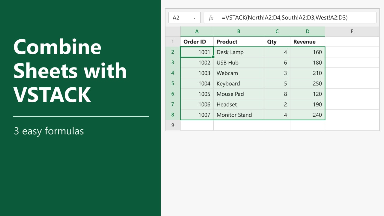
Copying and pasting rows from separate regional or monthly tabs into one master sheet every week quickly becomes tedious and error-prone. With a single dynamic array formula, you can stack rows from North, South, and West sheets into one live summary list that updates automatically when source data changes. In this tutorial, I'll show you how to combine multiple sheets with VSTACK in Excel using individual ranges, 3D references, and Excel Tables.
- Click cell A2 on your summary sheet below your column headers.
- To combine specific ranges from separate tabs, enter
=VSTACK(North!A2:D4, South!A2:D3, West!A2:D3)and press Enter. - To combine consecutive sheets with matching columns, use a 3D reference such as
=VSTACK(North:West!A2:D10)and filter out empty rows.
If your source tabs grow each week, format each sheet as an Excel Table (Method 3) so VSTACK picks up new rows automatically.
What Is the VSTACK Function in Excel?
The VSTACK function appends arrays vertically, placing the second range directly underneath the first in a single dynamic spill range. Its syntax is =VSTACK(array1, [array2], ...), where each argument is a cell range, Excel Table, or 3D sheet reference.
Version note: VSTACK requires Microsoft 365 (Windows, Mac, or Web) or Excel 2024. Older desktop versions such as Excel 2021 and Excel 2019 return a #NAME? error; if you use an older version, see our guide on combining sheets with Power Query or Consolidate.
All three methods below use the same sample workbook with three regional tabs (North, South, and West), each sharing four columns in A1:D1: Order ID, Product, Qty, and Revenue.
| Sheet | Data Range | Orders | Sample Rows |
|---|---|---|---|
| North | A1:D4 | 3 | 1001 Desk Lamp (160), 1002 USB Hub (180), 1003 Webcam (210) |
| South | A1:D3 | 2 | 1004 Keyboard (250), 1005 Mouse Pad (120) |
| West | A1:D3 | 2 | 1006 Headset (190), 1007 Monitor Stand (240) |
Method 1: Combine Specific Sheets with VSTACK
Use this approach when you want to combine two to five worksheets that are not next to each other or have different row counts. Our data sits in North!A2:D4, South!A2:D3, and West!A2:D3, with matching headers copied into A1:D1 on a blank Summary sheet.
- Open the Summary sheet and confirm row 1 holds your four headers in A1:D1.
- Select cell A2, leaving enough blank rows and columns below and to the right for all seven orders.
- Type the formula below into the formula bar.
- Press Enter to spill all seven rows from the three regional tabs into A2:D8.
=VSTACK(North!A2:D4, South!A2:D3, West!A2:D3)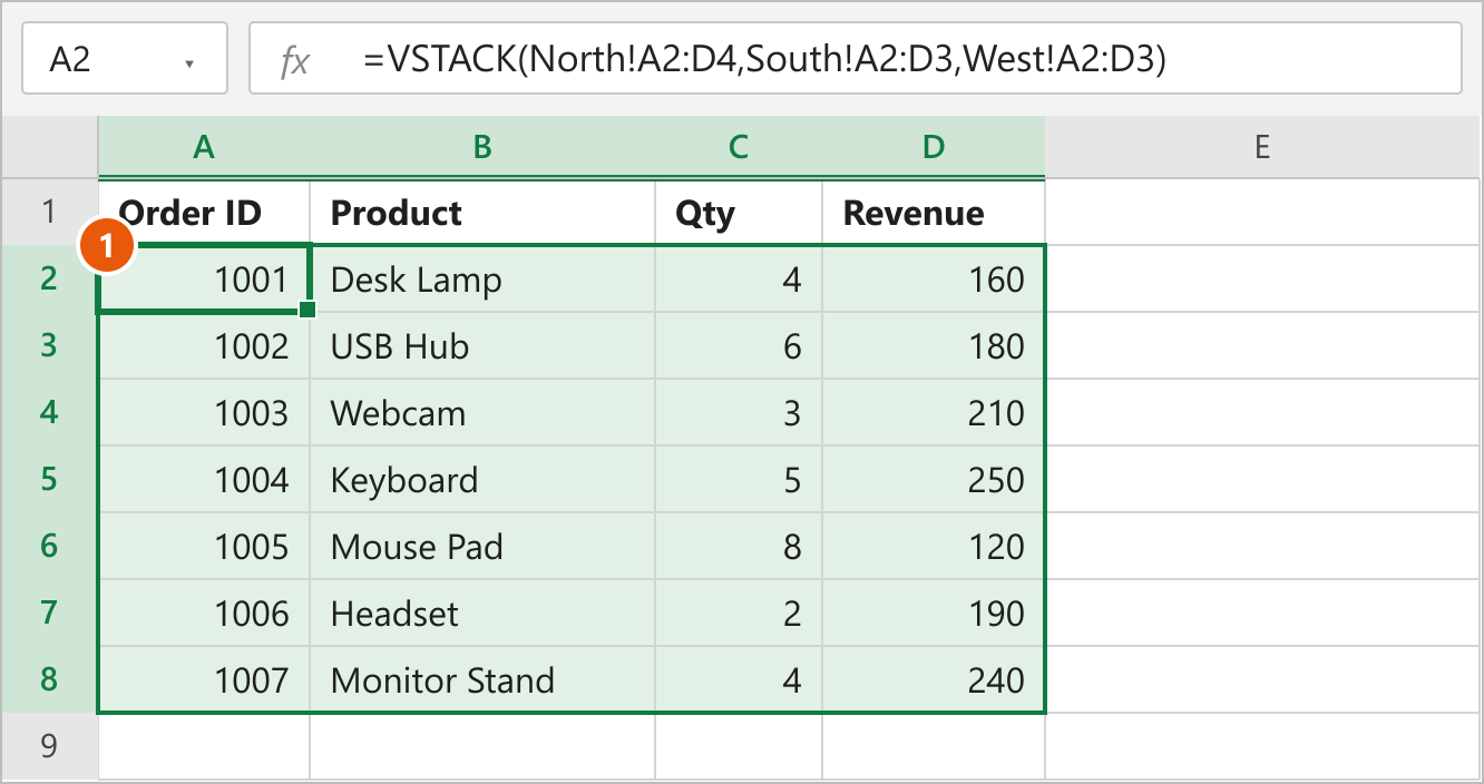
How this works: VSTACK reads North!A2:D4 first (orders 1001 to 1003), appends South!A2:D3 (orders 1004 and 1005), and finishes with West!A2:D3 (orders 1006 and 1007). Because the result is a dynamic array, editing any order on a regional tab updates Summary immediately.
Include Column Headers Automatically
You can pull the header row from the first tab instead of typing headers manually on Summary. Clear row 1, select cell A1, and include row 1 in the first range only.
=VSTACK(North!A1:D4, South!A2:D3, West!A2:D3)Note: If any cell inside the destination spill area already contains text, numbers, or spaces, Excel returns a #SPILL! error. Clear the blocking cells below A2 or check our troubleshooting steps to fix an Excel SPILL error.
Method 2: Combine Multiple Sheets with a 3D Reference and VSTACK
When you have many consecutive tabs with identical column layouts—such as monthly tabs from January to December—listing every sheet name by hand is slow. A 3D reference lets you specify only the first and last tab in the sequence.
Make sure the North, South, and West tabs sit next to each other in the workbook, and place Summary outside that span so it does not reference itself.
- Arrange your workbook tabs so North is first, South is in the middle, and West is last.
- Switch to the Summary sheet and select cell A2.
- Type the 3D formula below, replacing sheet names with single quotes if they contain spaces (for example,
'North Sales:West Sales'!A2:D4). - Press Enter to stack A2:D4 from all three tabs into A2:D10.
=VSTACK(North:West!A2:D4)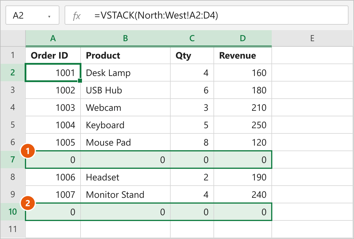
How this works: Excel evaluates the range A2:D4 on every worksheet sitting between North and West inclusive and stacks them in tab order. Any new tab you drag between North and West later is added automatically, while shorter sheets like South and West return 0 in row 4 because Excel converts empty cells inside array ranges to zeros.
Remove Blank Rows with LET, FILTER, and CHOOSECOLS
To reserve room for future orders without showing rows of zeros, reference a larger block such as A2:D10 and filter out rows where the first column is blank.
- Select cell A2 on your Summary sheet.
- Enter the formula below using a range taller than your largest source sheet, such as A2:D10.
- Press Enter to return only the seven populated rows in A2:D8.
=LET(d, VSTACK(North:West!A2:D10), FILTER(d, CHOOSECOLS(d, 1)<>""))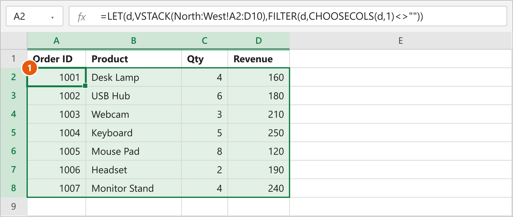
How this works: The LET function stores the stacked 3D array in a short variable named d so Excel calculates VSTACK once instead of twice. CHOOSECOLS(d, 1)<>"" checks column 1 (Order ID) for non-empty cells, and the FILTER function drops every empty row where that column was blank.
Note: CHOOSECOLS also requires Microsoft 365 or Excel 2024. Always point CHOOSECOLS to an identifier column that is never left blank on valid records.
Method 3: Combine Excel Tables with VSTACK for Dynamic Updates
If you add new orders to your regional sheets frequently, Excel Tables let VSTACK grow automatically with zero extra blank rows to filter out.
- Click any cell inside the data on the North tab and press Ctrl + T (Cmd + T on Mac) to create an Excel Table, keeping My table has headers checked.
- Go to Table Design > Table Name and name it NorthSales.
- Repeat the same steps on the South and West sheets, naming them SouthSales and WestSales.
- Switch to Summary, select cell A2, and enter the formula below.
- Press Enter to spill all seven rows into A2:D8.
=VSTACK(NorthSales, SouthSales, WestSales)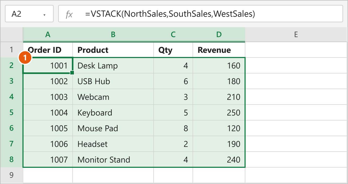
How this works: Named Excel Tables exclude their header rows by default when referenced by name, so VSTACK stacks only the data rows from NorthSales, SouthSales, and WestSales. Whenever you type a new order directly under any table, the table expands and the combined list on Summary updates right away.
If you also want to pull the header row dynamically into row 1 of Summary, enter =VSTACK(NorthSales[#Headers], NorthSales, SouthSales, WestSales) in cell A1.
Sort the Combined List or Handle Mismatched Columns
Once your sheets are stacked, wrap VSTACK inside SORT to order the master list by any column—for example, sorting descending by column 4 (Revenue) puts order 1004 (250) at the top.
=SORT(VSTACK(NorthSales, SouthSales, WestSales), 4, -1)If one sheet has fewer columns than the others, VSTACK fills the missing columns on the right with #N/A. Wrap the formula in IFNA to show blank cells instead of errors: =IFNA(VSTACK(NorthSales, SouthSales), ""). If your goal is a summarized report with totals rather than a raw row list, consider building a Pivot Table from multiple sheets instead.
FAQs
Does VSTACK work in Excel 2021 or Excel 2019?
Why does VSTACK show zeros when combining sheets?
Can VSTACK combine sheets with different numbers of columns?
Does VSTACK copy formatting from the source sheets?
How do I remove duplicates after stacking sheets with VSTACK?
Conclusion
For most workbooks where new rows are added every week, Method 3 (named Excel Tables inside VSTACK) is the cleanest setup because it expands without leaving zero rows behind. Use Method 2 with a 3D reference and FILTER when you have dozens of consecutive tabs that share one layout, and reach for Method 1 when you just need a quick formula across two or three sheets.