Use XLOOKUP with Multiple Criteria in Excel: Easy Guide

Sharing is caring!

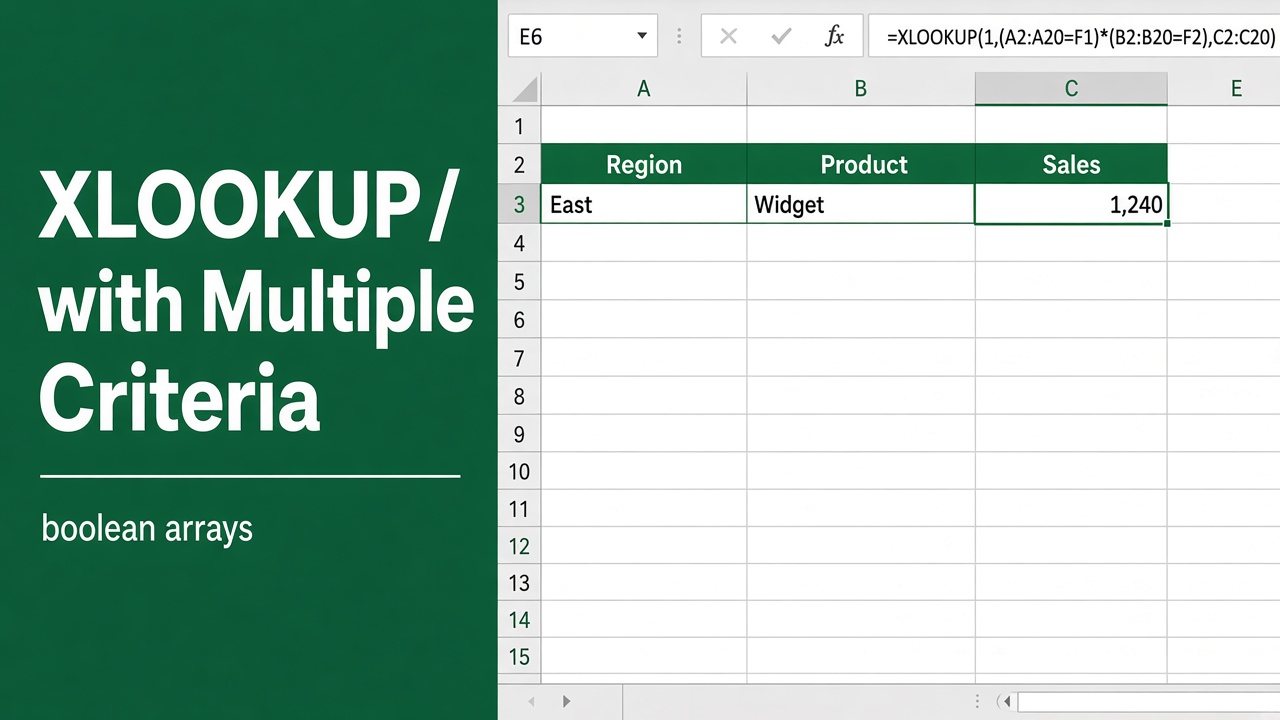
The XLOOKUP function in Excel is one of the most versatile tools for data retrieval. It allows users to search for values in a range or array and return corresponding results. But what if you need to base your search on multiple criteria?

In this article, we will provide a detailed guide on how to use XLOOKUP with multiple criteria, complete with examples, explanations, and practical tips.

Why Use Multiple Criteria in XLOOKUP?

In many real-world applications, a single lookup criterion may not be enough. Consider these scenarios:

• Retrieving the sales record of a specific product on a particular date.
• Finding the salary of an employee based on their department and job title.
• Locating student grades for a subject and exam type.

Using multiple criteria ensures precision, eliminates ambiguity, and enhances the accuracy of data retrieval.

Understanding the Syntax of XLOOKUP

Before we explore how to use XLOOKUP with multiple criteria, let’s revisit the basic syntax:

=XLOOKUP(lookup_value, lookup_array, return_array, [if_not_found], [match_mode], [search_mode])

• lookup_value: The value you want to search for.
• lookup_array: The range or array containing the lookup values.
• return_array: The range or array from which you want to return a value.
• if_not_found: The value to return if no match is found (optional).
• match_mode: Specifies exact or approximate matching (optional).
• search_mode: Defines the search direction (optional).

When using multiple criteria, we manipulate lookup_value and lookup_array to combine multiple conditions into a single array or helper column.

Methods to Use XLOOKUP with Multiple Criteria

Method 1: Combining Criteria with TEXTJOIN

The TEXTJOIN function is an excellent tool for combining multiple criteria into a single text string. This combined string can then be used as the lookup value.

Example: Finding Sales Data Based on Date and Product

Imagine this dataset:

You want to find the sales of Widget A on 01-Nov-24.

Steps:

1. Create a combined string for the lookup values:

=TEXTJOIN("-", TRUE, A2:A4, B2:B4) 

This generates an array: {"01-Nov-24-Widget A", "01-Nov-24-Widget B", "02-Nov-24-Widget A"}.

2. Combine the criteria for the lookup value:

 =TEXTJOIN("-", TRUE, "01-Nov-24", "Widget A")

3. Use XLOOKUP to search for the combined value:

 =XLOOKUP("01-Nov-24-Widget A", TEXTJOIN("-", TRUE, A2:A4, B2:B4), C2:C4)

Result:

The formula returns 500, corresponding to the sales of Widget A on 01-Nov-24.

Method 2: Using Helper Columns

Helper columns are one of the easiest and most efficient ways to implement multiple criteria in XLOOKUP. They simplify formulas and improve readability.

Example: Employee Lookup Based on Department and Job Title

Consider this dataset:

Steps:

1. Create a helper column by combining Department and Job Title:

=B2 & "-" & C2 

The helper column will look like this:

• Row 1: HR-Manager
• Row 2: IT-Developer
• Row 3: HR-Assistant

2. Use XLOOKUP to find the salary for an HR Manager:

=XLOOKUP("HR-Manager", D2:D4, E2:E4)

Result:

The formula returns 75,000, which is the salary of the HR Manager.

Method 3: Using Array Formulas

Array formulas allow dynamic matching without the need for helper columns. This approach uses Excel’s ability to process arrays directly in formulas.

Example: Retrieving Scores for a Student Based on Subject and Exam Type

Consider this dataset:

Steps:

1. Create an array formula using logical conditions:

=XLOOKUP(1, (B2:B4="Math")*(C2:C4="Final"), D2:D4)

• (B2:B4="Math") results in {TRUE, FALSE, TRUE}.
• (C2:C4="Final") results in {TRUE, FALSE, TRUE}.
• Multiplying these arrays gives {1, 0, 0}, which is used as the lookup value.

2. The XLOOKUP searches for 1 in the resulting array.

Result:

The formula returns 90, which is Mike’s Math final score.

Advantages of Using XLOOKUP with Multiple Criteria

1. Improved Accuracy: Combining criteria ensures precise data retrieval, reducing the risk of incorrect results.
2. Dynamic Functionality: XLOOKUP works seamlessly with arrays, allowing advanced data manipulation.
3. Versatility: It eliminates the need for older functions like INDEX-MATCH or nested IF formulas.
4. Error Handling: The if_not_found parameter simplifies error management.

Common Use Cases

1. Inventory Management: Retrieve stock quantities based on product name and warehouse location.
2. HR Analytics: Search for employee details using department and job title.
3. Academic Records: Fetch grades based on student name, subject, and exam type.
4. Financial Reports: Find transaction details using date and account number.

Troubleshooting and Common Errors

Comparison: XLOOKUP vs. VLOOKUP for Multiple Criteria

The table below compares XLOOKUP and VLOOKUP for handling multiple criteria:

Tips for Using XLOOKUP Effectively

1. Ensure Consistent Formatting: Avoid mismatches by formatting data in both the lookup and return arrays consistently.
2. Use Named Ranges: Replace range references with names to make formulas easier to read and manage.
3. Optimize for Large Data: Use helper columns or limit the size of lookup arrays to improve performance.

Final Thoughts

Mastering XLOOKUP with multiple criteria opens up a world of possibilities in Excel. Whether you’re managing inventory, analyzing employee data, or organizing academic records, this advanced technique ensures accuracy and efficiency. By leveraging functions like TEXTJOIN, helper columns, or array formulas, you can tailor your lookups to meet the most complex requirements.

Vaishvi Desai

Vaishvi Desai is the founder of Excelsamurai and a passionate Excel enthusiast with years of experience in data analysis and spreadsheet management. With a mission to help others harness the power of Excel, Vaishvi shares her expertise through concise, easy-to-follow tutorials on shortcuts, formulas, Pivot Tables, and VBA.