
Excel library
How to Remove Characters After a Dash Using Excel Formula?
Have you ever found yourself dealing with messy data in Microsoft Excel, filled with unnecessary characters after a dash? Tired of manually editing rows upon rows of information? Fortunately, there’s a solution that can streamline your data manipulation tasks and save you precious time.
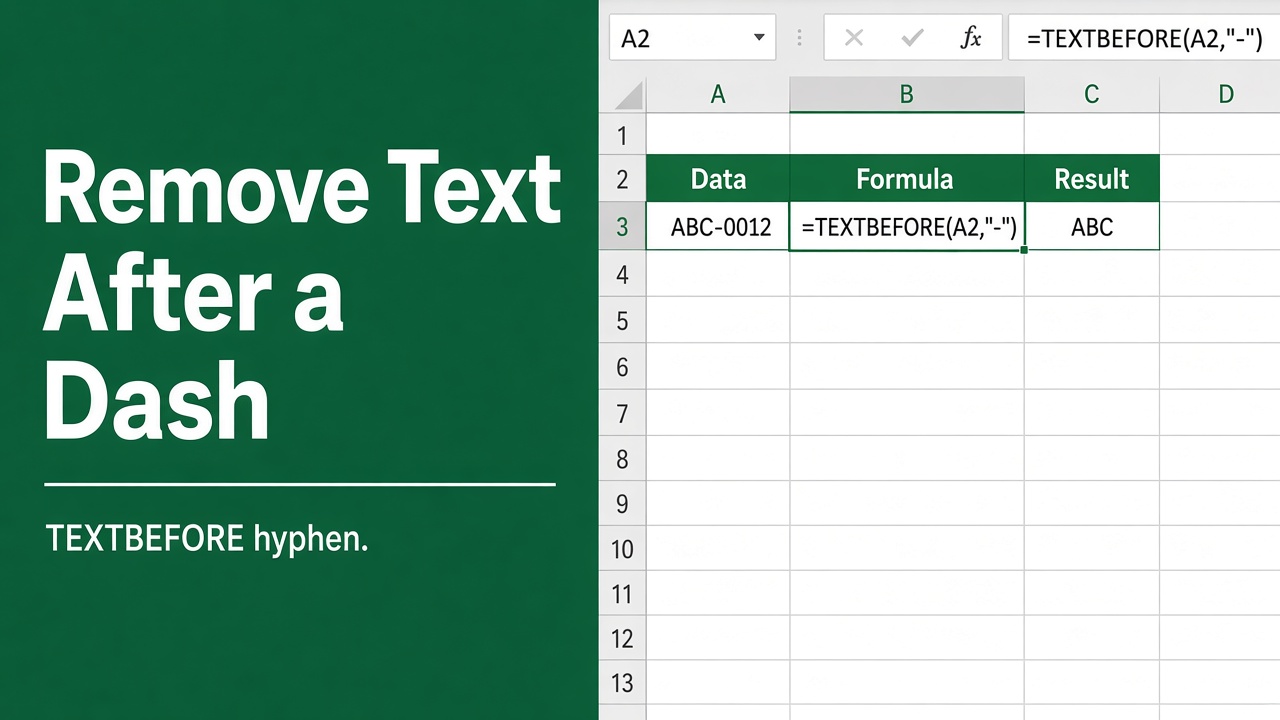
=TRIM(LEFT(A2, FIND("-", A2)-1))This keeps everything before the first dash (“Product A - Item 123” becomes “Product A”). Wrap it in IFERROR(..., A2) for cells without a dash. In Microsoft 365, =TEXTBEFORE(A2, "-") does the same, and =TEXTBEFORE(A2, "-", -1) cuts at the last dash. Without formulas: Ctrl + H, find -*, replace with nothing.
But how can you remove those unwanted characters quickly and efficiently using an Excel formula? In this article, we’ll guide you through the step-by-step process of removing characters after a dash in your Excel spreadsheets. With our expert tips and tricks, you’ll be able to extract valuable information and keep your data organized with ease. So, are you ready to take control of your data and simplify your workflow? Let’s get started!
Remove Everything After the Dash with LEFT and FIND
FIND returns the position of the dash, and LEFT keeps everything before it. With the text in A2:
=LEFT(A2, FIND("-", A2)-1)“Apple-Banana” becomes “Apple”. If there is a space before the dash, as in “Product A - Item 123”, wrap it in TRIM so the trailing space is removed too:
=TRIM(LEFT(A2, FIND("-", A2)-1))FIND returns #VALUE! when a cell has no dash. To return the original text in that case, use:
=IFERROR(TRIM(LEFT(A2, FIND("-", A2)-1)), A2)| Original Text (A) | Result |
|---|---|
| Apple-Banana | Apple |
| Product A - Item 123 | Product A |
| SKU-1001-RED | SKU |
| No dash here | No dash here |
Microsoft 365: TEXTBEFORE
In Microsoft 365 and Excel 2024, TEXTBEFORE does the same in one step:
=TRIM(TEXTBEFORE(A2, "-", , , , A2))The last argument returns the original text when there is no dash. To remove only what comes after the last dash, so “SKU-1001-RED” becomes “SKU-1001”, use -1 as the instance number: =TEXTBEFORE(A2, "-", -1).
Remove Only After the Last Dash (Any Version)
Without TEXTBEFORE, replace the last dash with a character that doesn’t appear in your data, such as ~, and cut there:
=LEFT(A2, FIND("~", SUBSTITUTE(A2, "-", "~", LEN(A2)-LEN(SUBSTITUTE(A2, "-", ""))))-1)LEN(A2)-LEN(SUBSTITUTE(A2, "-", "")) counts the dashes, so SUBSTITUTE changes only the last one.
You can also extract characters after a dash using formulas.
Keep the Text After the Dash Instead (MID)
To remove everything before the dash and keep what follows it:
=TRIM(MID(A2, FIND("-", A2)+1, LEN(A2)))“Product A - Item 123” becomes “Item 123”. In Microsoft 365, =TRIM(TEXTAFTER(A2, "-")) does the same.
Without a Formula: Find and Replace
- Select the cells and press Ctrl + H.
- In Find what, type
-*(a space, a dash and an asterisk). The asterisk is a wildcard for everything after the dash. - Leave Replace with empty and click Replace All.
This changes the original cells, so work on a copy. Note that SUBSTITUTE alone won’t do this job: =SUBSTITUTE(A2, "-", "") only deletes the dash itself and keeps the text after it.
When the Formula Can’t Find the Dash
Text copied from Word or web pages often contains an en dash (–) or em dash (—) instead of a hyphen (-). They look alike, but FIND(“-”) won’t match them. Either search for the actual character, =LEFT(A2, FIND("–", A2)-1), or convert them first with SUBSTITUTE(A2, "–", "-").
FAQ
How can I remove characters after a dash using an Excel formula?
Use =LEFT(A2, FIND("-", A2)-1). Wrap it in TRIM to remove a space before the dash, and in IFERROR(..., A2) to keep cells without a dash unchanged. In Microsoft 365, =TEXTBEFORE(A2, "-") does the same.
How do I remove everything after the last dash?
In Microsoft 365 use =TEXTBEFORE(A2, "-", -1). In older versions use =LEFT(A2, FIND("~", SUBSTITUTE(A2, "-", "~", LEN(A2)-LEN(SUBSTITUTE(A2, "-", ""))))-1).
How do I keep only the text after the dash?
Use =TRIM(MID(A2, FIND("-", A2)+1, LEN(A2))), or =TRIM(TEXTAFTER(A2, "-")) in Microsoft 365.
Can I remove text after a dash without a formula?
Yes. Select the cells, press Ctrl + H, type " -*" (space, dash, asterisk) in Find what, leave Replace with empty, and click Replace All. Flash Fill (type the first result and press Ctrl + E) also works.
Why does my formula return #VALUE!?
FIND can’t find the dash, either because the cell has none or because it contains an en dash (–) rather than a hyphen. Wrap the formula in IFERROR, or search for the en dash character instead.