How to Count Zeros in Excel Pivot Table Easily?

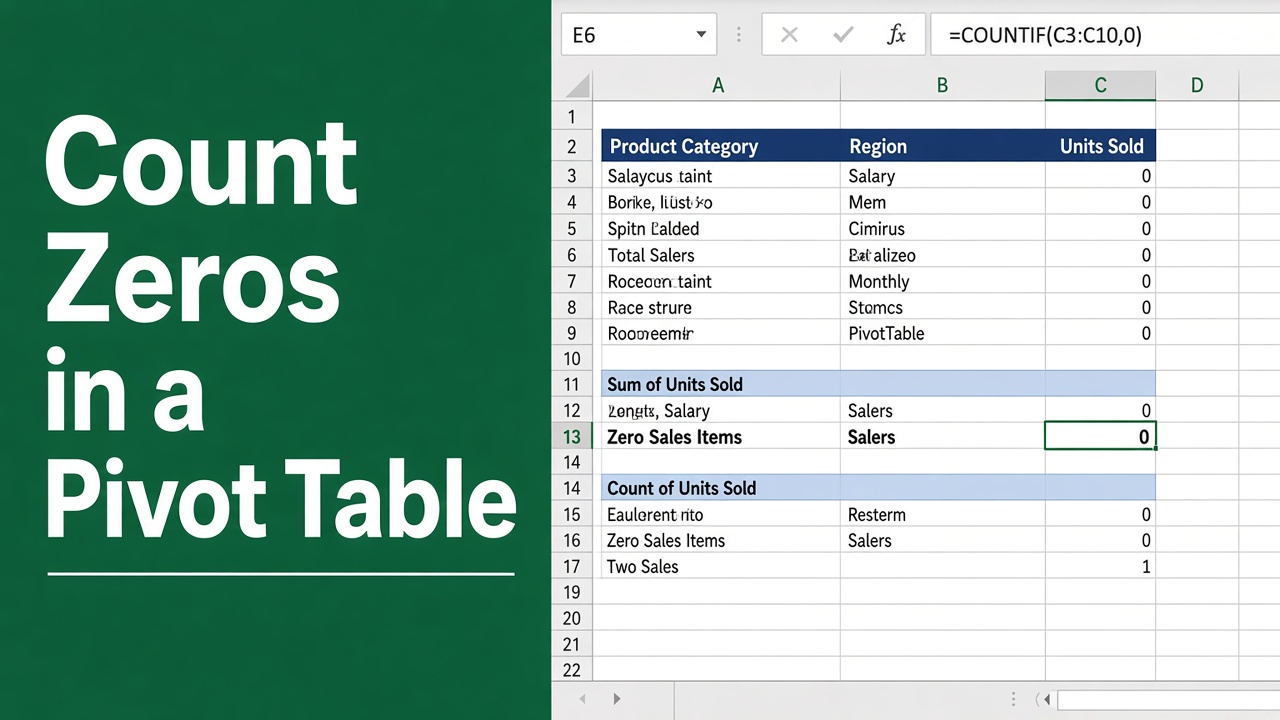
Are you working with an Excel pivot table and need to count the number of zeros in a specific field? Counting zeros in a pivot table can be a useful way to identify gaps in your data or to analyze trends. Whether you’re a business analyst, data scientist, or someone who works with large datasets, knowing how to count zeros in a pivot table is a valuable skill. In this comprehensive guide, we will walk you through the steps to easily count zeros in an Excel pivot table using simple formulas and built-in features.

Understanding Pivot Tables in Excel

Before we dive into counting zeros, let’s briefly discuss what a pivot table is and why it’s such a powerful tool in Excel.

What is a Pivot Table?

A pivot table is a feature in Excel that allows you to summarize, analyze, and explore large datasets. It enables you to quickly summarize data by different categories, calculate totals, averages, and other aggregate functions. Pivot tables are particularly useful when you have a large amount of data and need to extract meaningful insights from it.

Benefits of Using Pivot Tables

1. Data summarization: Pivot tables help you summarize large datasets into a concise and meaningful format. You can easily see the big picture and identify patterns or trends in your data.
2. Flexibility: With pivot tables, you can easily rearrange and filter data to gain insights from different perspectives. You can drag and drop fields to create different views of your data and explore it from various angles.
3. Automatic updates: When you update the source data, click Refresh (Alt + F5) and the pivot table recalculates with the new data, so you don’t need to rebuild your analysis.
4. Time-saving: Pivot tables save you a lot of time and effort compared to manually summarizing data using formulas or other methods. You can create a pivot table in just a few clicks and quickly generate reports or dashboards.

Preparing Your Data for a Pivot Table

To create a pivot table and count zeros effectively, you first need to ensure that your data is organized in a structured manner. One way to do this is by organizing your data into columns and rows, with clear headers and consistent formatting. Once your data is structured, you can easily create a pivot table in Excel or another data analysis tool. When counting zeros, it’s important to consider hiding blanks in the pivot table to accurately track the number of zeros in your data set. Hiding blanks in pivot table can help minimize any confusion and ensure that you are accurately counting the number of zeros in your dataset.

Data Structure Requirements

1. Consistent column headers: Each column in your dataset should have a unique header that clearly describes the data in that column. Avoid using blank headers or duplicate names.
2. No blank rows or columns: Remove any empty rows or columns within your dataset. Blank spaces can interfere with the creation and functionality of a pivot table.
3. Avoid merged cells: Unmerge any merged cells in your dataset, as they can cause issues when creating a pivot table. Each cell should contain an individual value.
4. Consistent data types: Ensure that the data in each column is of the same data type (e.g., numbers, text, dates). Mixed data types can lead to inconsistencies in the pivot table.

Once your data is properly structured, you’re ready to create a pivot table and start counting zeros.

Creating a Pivot Table in Excel

Creating a pivot table in Excel is a straightforward process. Here’s how you can do it:

1. Select any cell within your dataset.
2. Go to the Insert tab in the Excel ribbon.
3. Click on PivotTable in the Tables group.
4. In the Create PivotTable dialog box, ensure that the correct data range is selected. Excel usually detects the range automatically based on your selected cell.
5. Choose where you want to place the pivot table. You can create it in a new worksheet or an existing worksheet.
6. Click OK to create the pivot table.

Excel will create a blank pivot table based on your selected data range. You can now start arranging fields and exploring your data.

Counting Zeros in a Pivot Table

Now that you have created a pivot table, let’s explore different methods to count the number of zeros in a specific field.

Method 1: Filter the Field to Zero and Count

This works without changing your data. For example, to count the orders with a quantity of 0 for each region:

1. Drag the number field (e.g. Quantity) to the Filters area.
2. Drag the category (e.g. Region) to Rows.
3. Drag any field that is filled in on every row (e.g. Order ID) to Values and make sure it shows Count.
4. Click the filter dropdown above the pivot table, select 0, and click OK.

The pivot table now shows how many rows have a zero in each region. (Pivot table calculated fields can’t do this: they work on the summed values, not on individual rows, and there is no COUNTIF or PIVOTDATA function in a calculated field.)

Method 2: Using a Helper Column

If you prefer not to use a calculated field, you can add a helper column to your source data to count the zeros. This method involves modifying your original dataset before creating the pivot table.

1. In your source data, insert a new column next to the field you want to count zeros for.
2. In the new column, enter the following formula: =IF(B2=0,1,0), replacing B2 with the cell reference of the first data point in the field you want to count zeros for.
3. Drag the formula down to apply it to the entire column. This formula will put a 1 in the helper column if the corresponding value in the original field is zero, and a 0 otherwise.
4. Create a pivot table using your updated source data.
5. Drag the helper column into the Values area of the pivot table.
6. The pivot table will now display the count of zeros for the selected field based on the helper column.

Using a helper column can be useful if you want to preserve the original data and perform additional calculations or analysis based on the count of zeros.

Advanced Techniques for Counting Zeros

Counting Zeros in Multiple Fields

Add one helper column per field, such as =--(C2=0) for Jan and =--(D2=0) for Feb, and drag each helper into the Values area as Sum. To count rows where any of several columns is zero, use one helper: =--(COUNTIF(C2:F2, 0)>0).

Conditional Counting of Zeros

Put the condition in the pivot table rather than the formula: keep the helper column =--(B2=0), then drag the condition field (for example Status) to the Filters area or Columns area. Outside a pivot table, =COUNTIFS(B:B, 0, C:C, "East") counts the zeros in column B where column C is “East”.

Note that blank cells aren’t zeros: COUNTIF(B:B, 0) and the helper formulas ignore empty cells. Use =--(B2="") to count blanks separately.

Best Practices for Counting Zeros in Pivot Tables

To ensure accurate and reliable results when counting zeros in pivot tables, consider the following best practices:

1. Ensure data accuracy: Before counting zeros, double-check your source data for any errors, inconsistencies, or missing values. Clean and validate your data to avoid skewed results.
2. Use meaningful names: When creating calculated fields or helper columns, use descriptive and meaningful names that clearly indicate their purpose. This makes it easier for you and others to understand the analysis later on.
3. Refresh pivot tables: If you make changes to your source data, remember to refresh your pivot table to update the zero counts. Right-click on the pivot table and select Refresh to ensure the data is up to date.
4. Verify the results: Always cross-check the zero counts in your pivot table with the actual data to ensure accuracy. Spot-check a few values to confirm that the calculations are correct.
5. Document your steps: Keep track of the formulas, calculated fields, and any modifications you make to your pivot table. Document your analysis steps for future reference and to maintain transparency.
6. Use appropriate formatting: Apply appropriate number formatting to your pivot table fields to display the zero counts correctly. Use commas, decimal places, or other formatting options as needed.

By following these best practices, you can ensure that your zero count analysis in pivot tables is accurate, reliable, and easily understandable.

Final Thoughts

Counting zeros in an Excel pivot table is a powerful technique for analyzing and exploring large datasets. Whether you’re identifying gaps in your data, examining trends, or making data-driven decisions, counting zeros provides valuable insights.

Remember to structure your data properly, use meaningful names for calculated fields, refresh your pivot tables when needed, and verify your results to ensure accuracy. By mastering the art of counting zeros in pivot tables, you can unlock the full potential of your data and make informed decisions with confidence.

FAQs