
Excel library
How to COUNTIF with Multiple Criteria in Excel (4 Easy Ways)
You have a sales list and need to know how many orders came from the East region and were for laptops, but COUNTIF only accepts one condition. The fix is to count rows that pass two or more tests at once, either all of them (AND) or any of them (OR). In this tutorial, I'll show you how to COUNTIF in Excel with multiple criteria using four formulas, from the simple COUNTIFS to SUMPRODUCT.
- Use COUNTIFS and give it one range and one condition per test:
=COUNTIFS(B2:B9,"East",C2:C9,"Laptop"). - For OR logic in one column, wrap COUNTIF in SUM with a list:
=SUM(COUNTIF(B2:B9,{"East","West"})).
COUNTIFS (Method 1) covers most cases, because every condition must be true at the same time.
All four methods use the same small table. It has 8 orders in A1:D9, with the sales rep in column A, the region in column B, the product in column C and the units sold in column D.
| Rep | Region | Product | Units |
|---|---|---|---|
| Anna | East | Laptop | 12 |
| Ben | West | Phone | 30 |
| Chloe | East | Phone | 18 |
| David | North | Laptop | 7 |
| Ella | West | Laptop | 25 |
| Frank | East | Laptop | 40 |
| Grace | North | Phone | 15 |
| Henry | West | Phone | 9 |
Method 1: Using the COUNTIFS Function (AND Criteria)
Use COUNTIFS when a row should only be counted if it meets every condition. It is the multi-criteria version of the COUNTIF formula and works in Excel 2007 and later.
COUNTIFS syntax
=COUNTIFS(criteria_range1, criteria1, [criteria_range2, criteria2], ...)Each condition is a pair: the range to check and the value to look for. You can add up to 127 pairs.
Here we want the number of orders that are from the East region and for a Laptop.
- Select cell G2.
- Type =COUNTIFS( to start the function.
- Enter B2:B9,"East" as the first range and condition.
- Add a comma, then C2:C9,"Laptop" as the second pair.
- Close the bracket and press Enter.
=COUNTIFS(B2:B9,"East",C2:C9,"Laptop")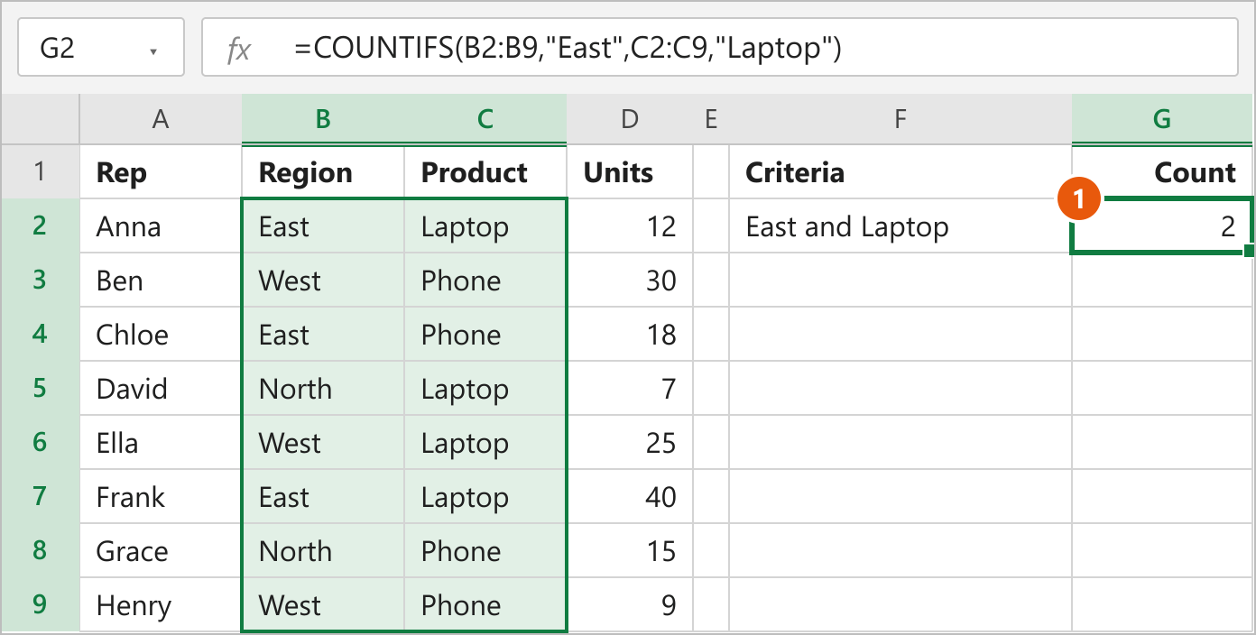
How this works: COUNTIFS checks each row against both conditions. A row is counted only when column B says East and column C says Laptop on the same row. Anna and Frank pass both tests, so the result is 2. Chloe is in the East but sold a phone, so she is left out.
Note: Every range must be the same size. If one range is B2:B9 and another is C2:C10, COUNTIFS returns a #VALUE! error. Text criteria are not case-sensitive, so "east" and "East" give the same count.
Method 2: Using COUNTIFS with Comparison Operators
Conditions don't have to be exact matches. You can use operators such as >, <, >=, <= and <> (not equal to) to count numbers in a range or exclude a value.
To count orders with between 10 and 30 units, you check column D twice, once for each limit.
- Select cell G2.
- Type the formula below. The operator and number go inside quotes.
- Press Enter.
=COUNTIFS(D2:D9,">=10",D2:D9,"<=30")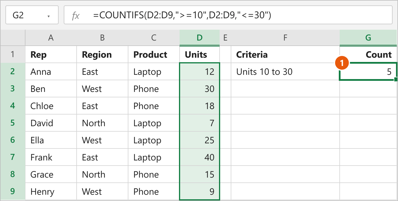
How this works: The first pair keeps units of 10 or more, and the second keeps units of 30 or less. Only values that pass both are counted: 12, 30, 18, 25 and 15. That gives 5. Frank's 40 and the two orders below 10 are excluded. There's a full guide on this pattern if you want to count between two numbers in Excel.
Using cell references as criteria
Typing values into the formula works, but putting them in cells lets you change the criteria without editing the formula. In this example, G2 holds the region and G3 holds the minimum units.
- Type West in cell G2.
- Type 20 in cell G3.
- Select cell G4 and enter the formula below.
=COUNTIFS(B2:B9,G2,D2:D9,">="&G3)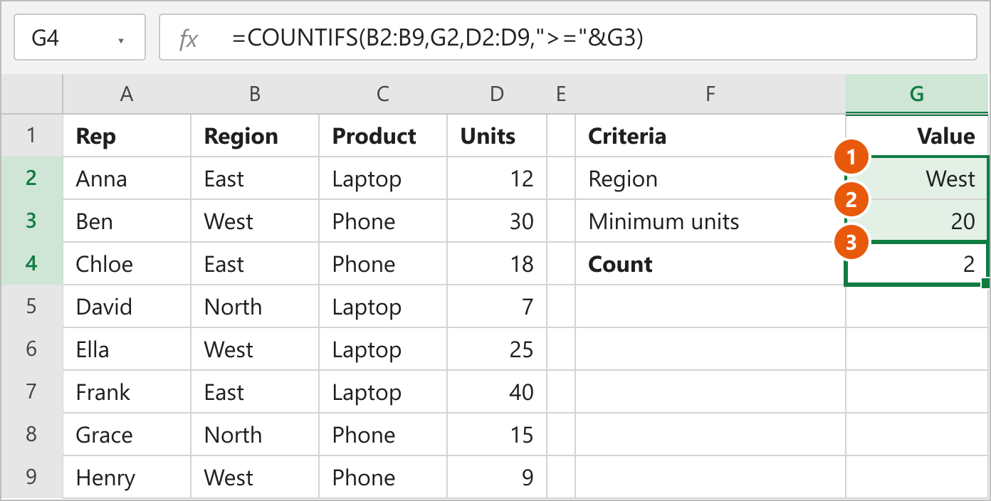
For an exact match, the cell reference goes in on its own. When you need an operator, keep the operator in quotes and join it to the cell with &. Writing ">=G3" would not work, because Excel would read G3 as text. Ben (30) and Ella (25) are the West orders with at least 20 units, so the result is 2.
Method 3: Using SUM and COUNTIF for OR Criteria
COUNTIFS always joins conditions with AND. When you want rows that match one value or another in the same column, use COUNTIF with an array constant (a list of values in curly braces) and add up the results with SUM.
- Select cell G2.
- Type the formula below, with the regions you want inside { }.
- Press Enter.
=SUM(COUNTIF(B2:B9,{"East","West"}))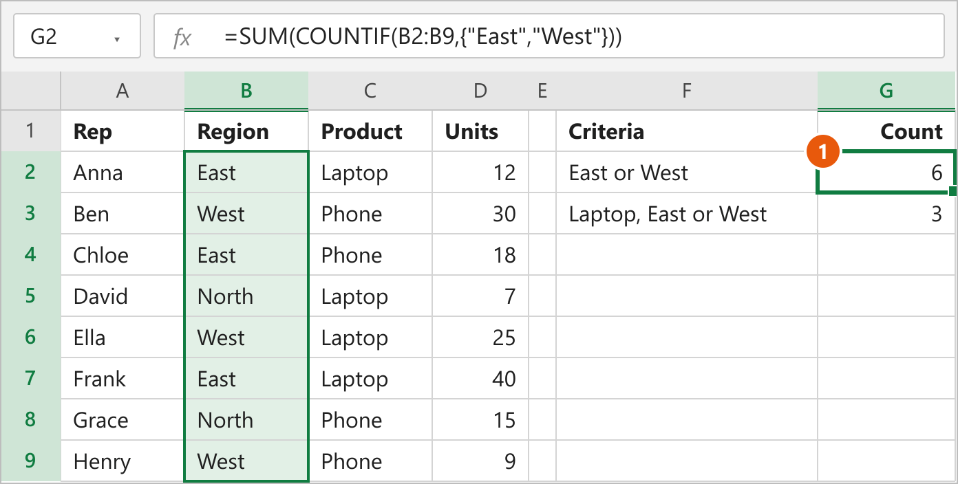
How this works: COUNTIF runs once for each item in the list. It returns 3 for East and 3 for West. SUM adds them together to get 6. You type the braces yourself, and the formula works with a normal Enter in every version of Excel.
Combining OR and AND
The same trick works with COUNTIFS. To count laptops sold in either the East or the West, enter this in G3:
=SUM(COUNTIFS(B2:B9,{"East","West"},C2:C9,"Laptop"))It returns 3: Anna and Frank in the East, plus Ella in the West. That is the value shown in G3 in the screenshot above.
Note: This method is only safe when the OR values are in one column. A row can't be East and West at the same time, so nothing is counted twice. For OR conditions across different columns, use Method 4.
Method 4: Using SUMPRODUCT for OR Across Columns
Say you want orders that are from the East or have more than 20 units. Adding two COUNTIF results would give 3 + 3 = 6, but Frank meets both conditions and would be counted twice. SUMPRODUCT lets you count each row once.
- Select cell G2.
- Type the formula below.
- Press Enter.
=SUMPRODUCT(--(((B2:B9="East")+(D2:D9>20))>0))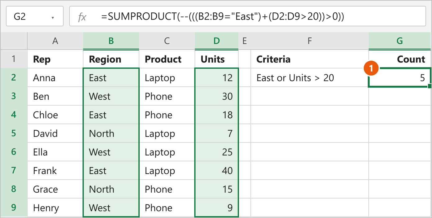
How this works: Each test in brackets returns TRUE or FALSE for every row. Adding the two tests turns them into numbers: 0 if a row fails both, 1 if it passes one, and 2 if it passes both. The >0 check turns any row with 1 or 2 back into TRUE. The double minus (--) converts TRUE to 1 and FALSE to 0, and SUMPRODUCT adds them up. Anna, Ben, Chloe, Ella and Frank qualify, so the answer is 5.
For AND logic in SUMPRODUCT, multiply the tests instead of adding them: =SUMPRODUCT((B2:B9="East")*(C2:C9="Laptop")) returns 2, the same as Method 1.
Note: SUMPRODUCT does not support wildcards like * the way COUNTIFS does, and it can slow down on very large ranges. Avoid whole-column references such as B:B inside it.
FAQs
Can COUNTIF have multiple criteria?
What is the difference between COUNTIF and COUNTIFS?
Why does my COUNTIFS formula return #VALUE!?
Can I use wildcards with COUNTIFS?
How do I count cells that are not equal to a value?
Conclusion
For most multi-criteria counts, COUNTIFS is the one to use. It is easy to read, handles operators and wildcards, and every condition must be true for a row to count. Switch to SUM with COUNTIF when you need OR logic inside a single column. Keep SUMPRODUCT for OR conditions that span different columns, where adding separate counts would count some rows twice. If you also need totals rather than counts, the same ideas apply to SUMIF with multiple criteria.