
Excel library
How to Move Columns in Excel (4 Easy Ways)
You get a report where the column you care about sits at the far right, or a template that puts Region before Sales when your boss wants it the other way round. Moving a column means shifting all its cells to a new position while the other columns slide over to make room, without overwriting anything.
Excel has no single "Move Column" button, but it offers several quick ways to do it. In this tutorial, I'll show you how to move columns in Excel using drag and drop, cut and insert, sorting, and a formula.
- Click the column letter to select the whole column.
- Hover over the edge of the selection until the cursor turns into a four-headed arrow.
- Hold Shift, drag the column to its new position, and release the mouse before you release Shift.
If dragging feels fiddly, use cut and Insert Cut Cells from Method 2 instead.
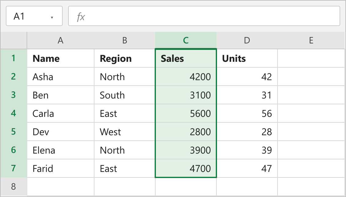
Our data is in A1:D7: names in column A, regions in B, sales in C and units in D. In most examples we want Sales to sit right after Name, before Region.
Method 1: Using Shift and Drag to Move Columns in Excel
This is the fastest way to move one column, or a block of side-by-side columns, a short distance.
- Click the column letter C to select the Sales column.
- Move the pointer to the left or right edge of the selection until it becomes a four-headed arrow.
- Press and hold Shift.
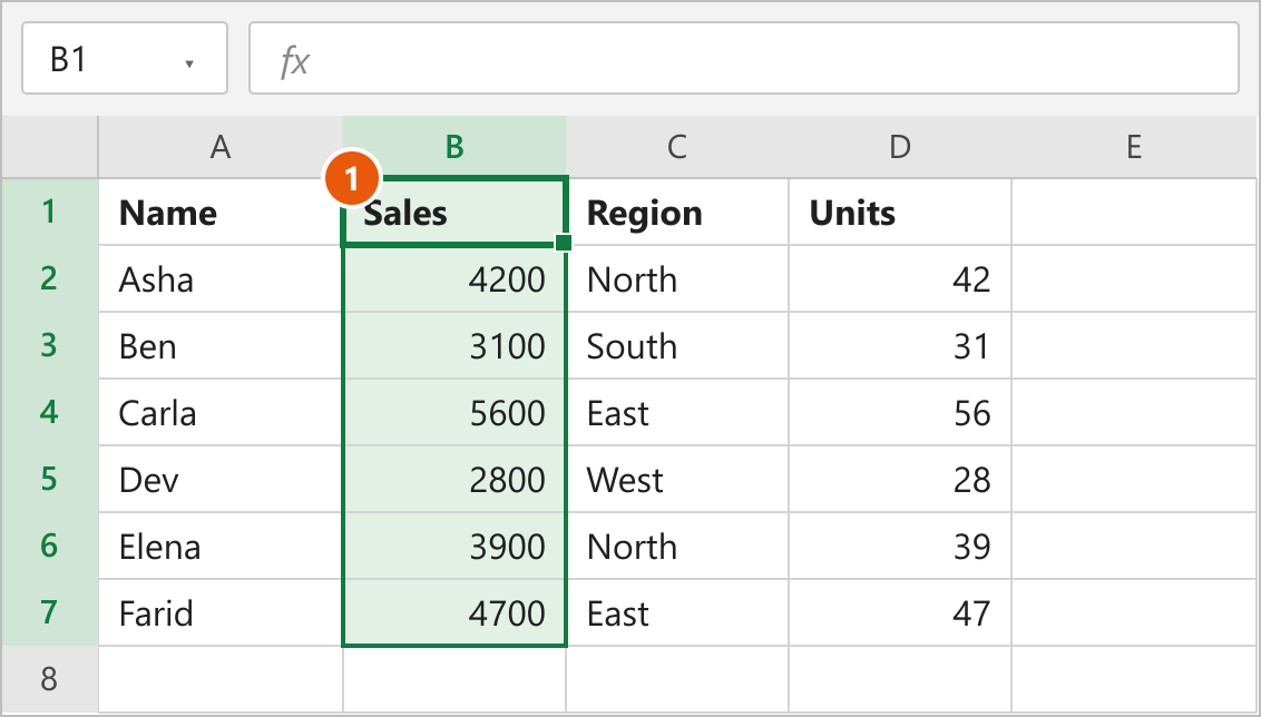
- Drag to the left. A thick green line shows where the column will land. Stop when it sits between columns A and B.
- Release the mouse button first, then release Shift.
Sales is now in column B, and Region and Units each shift one column to the right.
How this works
A normal drag moves cells on top of whatever is already there. Holding Shift changes it to an insert, so Excel opens a gap at the green line and pushes the other columns aside. Formulas that refer to the moved cells update automatically.
Note: If you forget to hold Shift, Excel asks "There's already data here. Do you want to replace it?" Click Cancel and try again with Shift held down.
Method 2: Using Cut and Insert Cut Cells
Use this when the column has to travel far, for example from column Z to column B, where dragging means scrolling. This time we move Units from column D to column B.
- Right-click the column letter D and choose Cut, or select the column and press Ctrl+X.
- Right-click the column letter B. The cut column will land to the left of this column.
- Choose Insert Cut Cells from the menu.
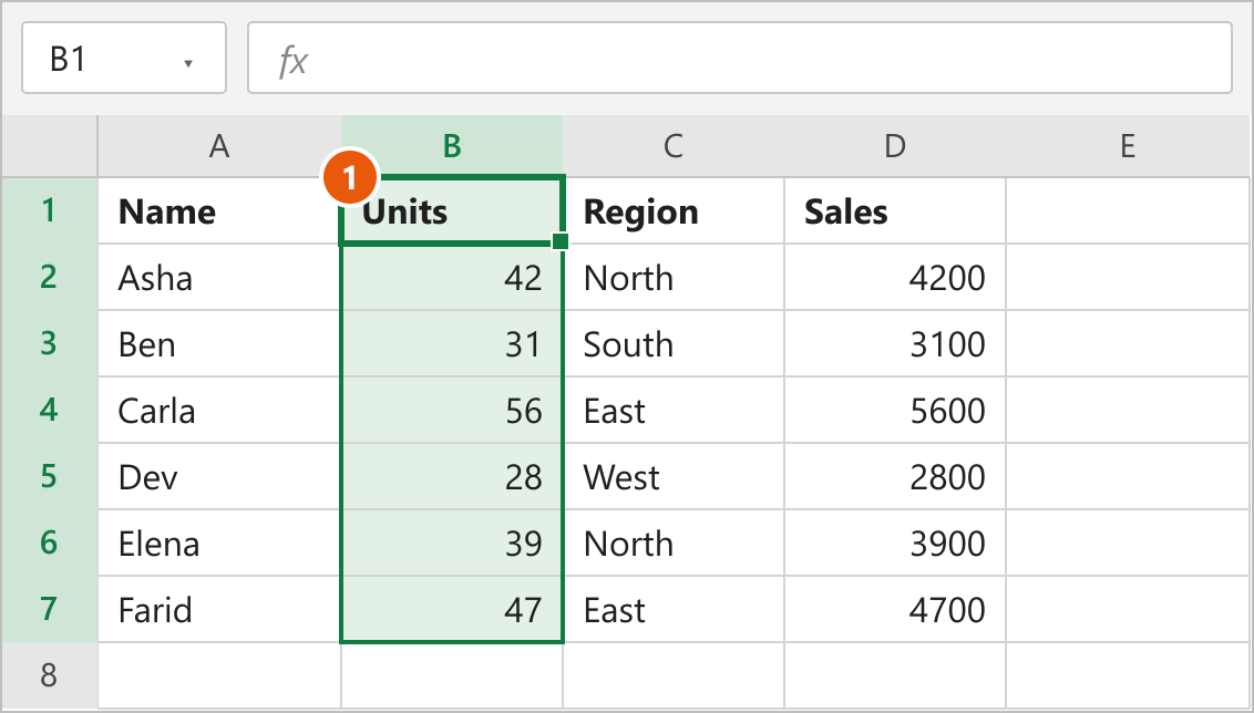
Units moves into column B, and Region and Sales shift right to C and D.
Keyboard-only version
Select a cell in column D, press Ctrl+Space to select the whole column, and press Ctrl+X. Click any cell in column B, press Ctrl+Space again, and then press Ctrl+Shift+Plus (Ctrl+Shift+=) to insert the cut column there. If you use cut often, our guide to the keyboard shortcut to cut a cell in Excel covers it in more detail.
How this works
Cut marks the column with a moving dotted border but does not remove anything yet. Insert Cut Cells then removes the column from its old spot and inserts it at the new one in one step. If you choose Paste instead, Excel overwrites column B rather than inserting.
Method 3: Using Sort Left to Right to Rearrange Many Columns
When you need to reorder many columns at once, moving them one by one is slow. Instead, number the columns in the order you want and let Excel sort them sideways.
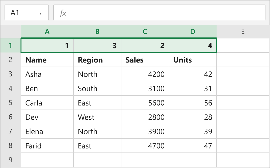
- Insert a blank row above the headers, so the table now runs from A2 to D8.
- In row 1, type the position each column should end up in: 1 for Name, 3 for Region, 2 for Sales and 4 for Units.
- Select A1:D8, then go to Data and click Sort.
- Click Options, select Sort left to right, and click OK.
- Set Sort by to Row 1 and Order to Smallest to Largest, then click OK.
- Delete row 1 once the columns are in place.
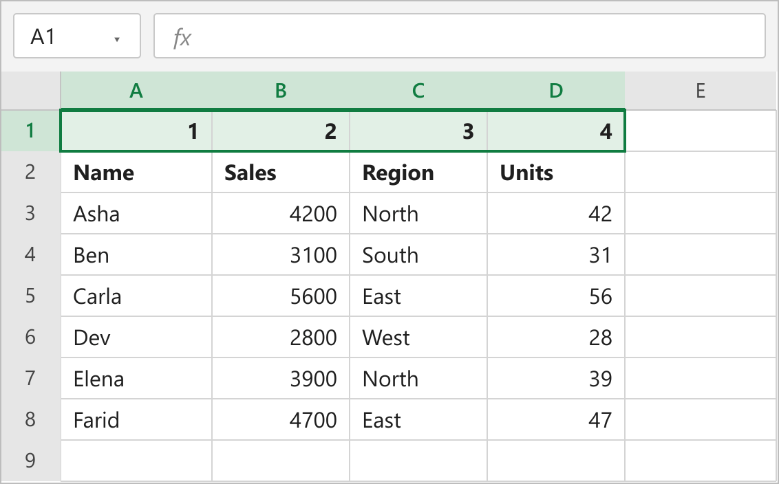
After the sort, row 1 reads 1, 2, 3, 4 and the headers read Name, Sales, Region, Units.
How this works
A normal sort reorders rows by the values in one column. Sort left to right does the same thing sideways: it reorders whole columns by the values in one row. Because row 1 holds the positions you typed, the columns end up in exactly that order.
Note: Select only the table, not whole rows. If the selection includes columns you did not number, Excel sorts the blank cells to the end and can move columns you meant to leave alone.
Method 4: Using the CHOOSECOLS Function
Use this when you want a reordered copy of the table and need to keep the original as it is, for example on a report sheet. CHOOSECOLS is available in Microsoft 365 and Excel 2024.
- Select cell F1.
- Type the formula below.
- Press Enter.
=CHOOSECOLS(A1:D7,1,3,2,4)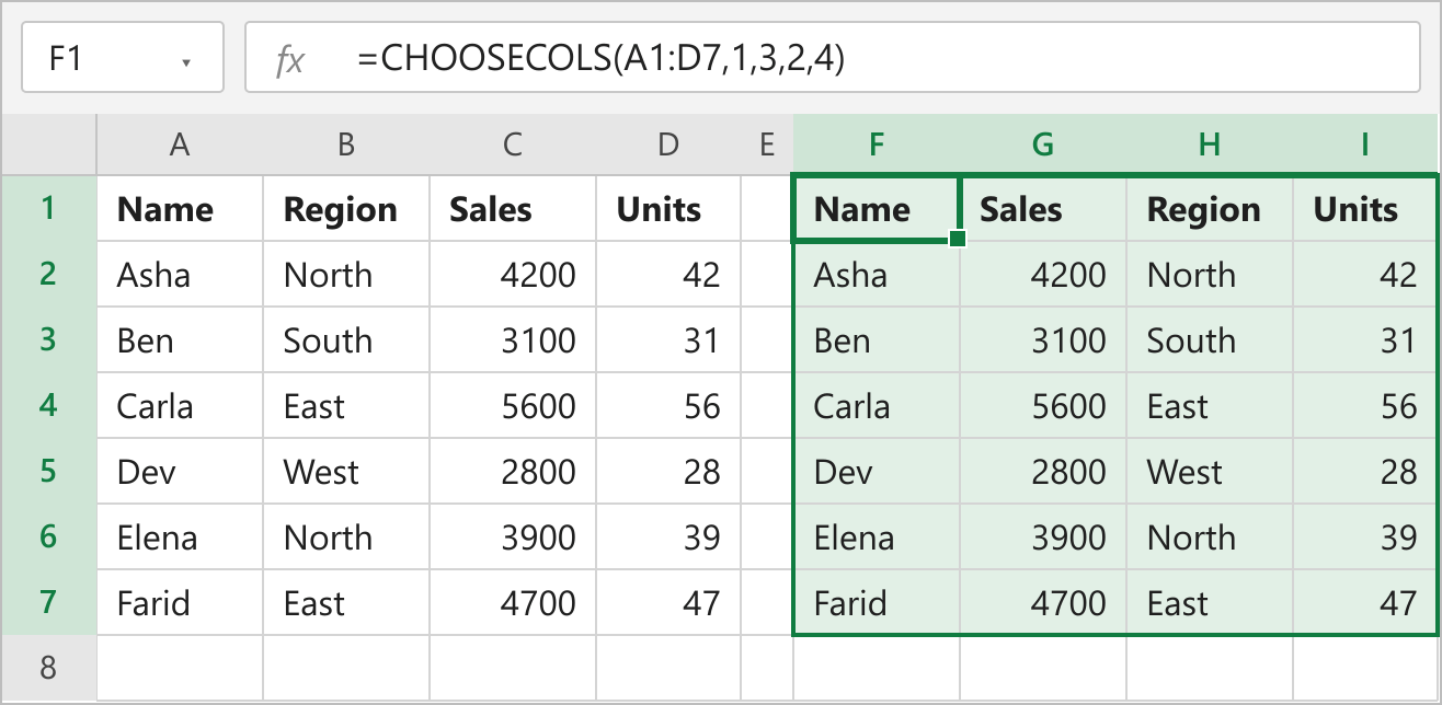
How this works
CHOOSECOLS takes a range and a list of column numbers, and returns those columns in the order you list them. Here 1, 3, 2, 4 means Name, Sales, Region, Units. The result spills into F1:I7 and updates whenever the source data changes.
Note: The spilled copy is a formula result, so you cannot edit single cells in it. To get plain values, copy F1:I7 and use Paste Values.
FAQs
Will moving a column break my formulas?
Can I move several columns at once?
Why does Excel say "This action won't work on multiple selections"?
Do these methods work inside an Excel table?
How do I move columns in a pivot table?
Conclusion
For one column moving a short distance, Shift + drag is the quickest, and it is the method I would use most of the time. Use cut and Insert Cut Cells when the column has a long way to go, and sort left to right when you need to reorder many columns at once. Choose CHOOSECOLS when the original layout has to stay untouched.